Tag: Nodes

Trade Network Updates, Part 2 (node code)

Over the last 10 days I’ve been playing around with code that will enable some new versions of the MLB trade networks I premiered way back in 2015. The goal this time around is to factor in the future value of a trade to each of the participating teams. There are multiple measures that could be used for this assessment but I’m going with the WAR162 value from Neil Paine’s 538 github data source. Here’s how the site describes the War162 measure: JEFFBAGWELL WAR per 162 team games. Now you may ask why Jeff Bagwell? While he was a talented hitter for many years, his name is used as an acronym for this:

“The file “jeffbagwell_war_historical.csv” contains wins above replacement (WAR) data — according to JEFFBAGWELL (the Joint Estimate Featuring FanGraphs and B-R Aggregated to Generate WAR, Equally Leveling Lists), which averages together WAR from Baseball-Reference.com and FanGraphs — plus various other metrics for MLB since 1901.” Fun stuff, right?

The bottom line from my perspective is that this measure provides a robust way of assessing the value of a trade based on performance after the trade date. Did one team benefit while another team received a player who added no future value? Or did both teams make out equally well? Or was the trade of minimal value for both sides? These are the questions I’m attempting to visually address using network analysis and visualization.

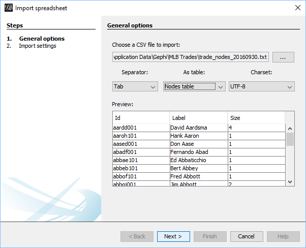
Now comes the technical aspect for all you database and code lovers. First step is to create the network nodes; in this case we need to display the individual trade transactions, teams, and players. Let’s look first at the transactions using the Visual-Baseball MySQL source data:

SELECT CONCAT(a.Id, ‘-‘, a.PrimaryDate) as Id, CONCAT(‘Transaction ‘,a.Id,’ is from the ‘, a.Season, ‘ season’) AS Label,
‘Trade’ AS Type, SUM(a.Size) AS Size
FROM
(SELECT tr.TransactionID AS Id, tr.Season, tr.PrimaryDate, ROUND(SUM(h.WAR162),1) as Size
FROM historical_WAR_and_more h
INNER JOIN People p
ON h.key_bbref = p.bbrefID
INNER JOIN trades2021 tr
ON p.retroID = tr.Player
INNER JOIN Teams t
ON tr.TeamTo = t.teamID

WHERE tr.Season >= 1901 and h.year_ID >= tr.season and tr.Type = ‘T’ and tr.TeamTo = t.teamID and LENGTH(tr.TeamFrom) = 3
AND tr.Season = t.yearID and t.franchID = h.franch_ID

GROUP BY tr.TransactionID, tr.season, tr.TeamFrom, tr.TeamTo, tr.PrimaryDate) a

GROUP BY a.Id, a.PrimaryDate, a.Season;

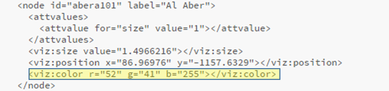
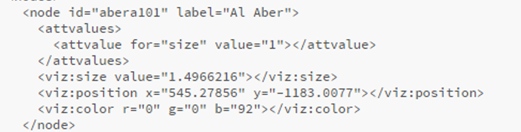
Here we are simply creating a node for each trade transaction, a label showing the teams involved and the trade date, and summing up the previously mentioned WAR162 to size the nodes. This will be an important part of the graph – trades that created large future values (for one or both teams) will be more prominent in the graph. Small value trades will be represented by very small nodes indicating their relative lack of importance. This one was a challenge, but finally got the code to deliver the expected results.

The next step is to create team nodes; in this case we’ll provide a constant size:

SELECT t.franchID AS Id, tf.franchName AS Label, 15 AS Size

FROM historical_WAR_and_more h
INNER JOIN People p
ON h.key_bbref = p.bbrefID
INNER JOIN trades2021 tr
ON p.retroID = tr.Player
INNER JOIN Teams t
ON tr.TeamFrom = t.teamID
INNER JOIN TeamsFranchises tf
ON t.franchID = tf.franchID

WHERE tr.season >= 1901 and h.year_ID >= tr.season and tr.Type = ‘T’ and h.team_ID = tr.TeamTo and LENGTH(tr.TeamFrom) = 3

GROUP BY t.franchID, tf.franchName;

By applying a constant node size of 15, each team will have a similar appearance in the graph which will not distract us from the trade values (some will be much larger than 15).

Our third and final node step is to provide information on all players involved in one or more trades:

SELECT Id, Label, ‘Player’ AS Type, 5 AS Size
FROM
(SELECT p.playerID AS Id,
CONCAT(h.player_name, ‘ (‘, p.birthYear,’-‘,p.deathYear,’)’,’ played from ‘,LEFT(p.debut,4),’ to ‘,LEFT(p.finalGame,4)) AS Label

FROM historical_WAR_and_more h
INNER JOIN People p
ON h.key_bbref = p.bbrefID
INNER JOIN trades2021 tr
ON p.retroID = tr.Player

WHERE tr.season >= 1901 and h.year_ID >= tr.season and tr.Type = ‘T’ and LENGTH(tr.TeamFrom) = 3
and LENGTH(tr.TeamTo) = 3
AND p.deathYear > 1900

GROUP BY h.player_name, p.playerID, p.birthYear, p.deathYear, p.debut, p.finalGame

UNION ALL

SELECT p.playerID AS Id,
CONCAT(h.player_name, ‘ (‘, p.birthYear,’-‘,’ )’,’ played from ‘,LEFT(p.debut,4),’ to ‘,LEFT(p.finalGame,4)) AS Label

FROM historical_WAR_and_more h
INNER JOIN People p
ON h.key_bbref = p.bbrefID
INNER JOIN trades2021 tr
ON p.retroID = tr.Player

WHERE tr.season >= 1901 and h.year_ID >= tr.season and tr.Type = ‘T’ and LENGTH(tr.TeamFrom) = 3
and LENGTH(tr.TeamTo) = 3
AND ISNULL(p.deathYear)

GROUP BY h.player_name, p.playerID, p.birthYear, p.deathYear, p.debut, p.finalGame) a
GROUP BY Id, Label;

Here we are running a UNION query so we can gather information about the players moving in each direction of a trade (from one team to another). We then combine that information and apply a fixed size of 5 since there are far more players than teams. We’ll have the ability in the finished networks to zoom in and see more about each player.

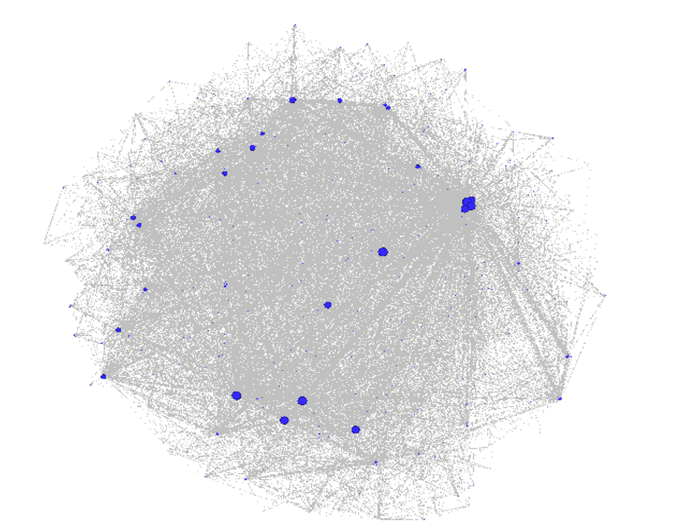
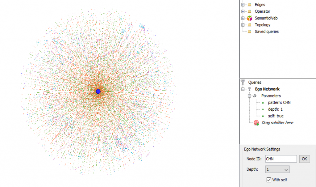
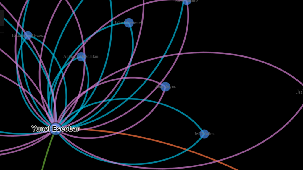
Each of these 3 outputs (trades, teams, and players) is combined into a single input file that will feed Gephi. We should wind up with between 10k and 20k nodes which we’ll be able to filter
and zoom on in the network graph. I have high hopes for this set of networks (there may be one for each team as well as a comprehensive one) as it should really help display the most important trades in MLB history.

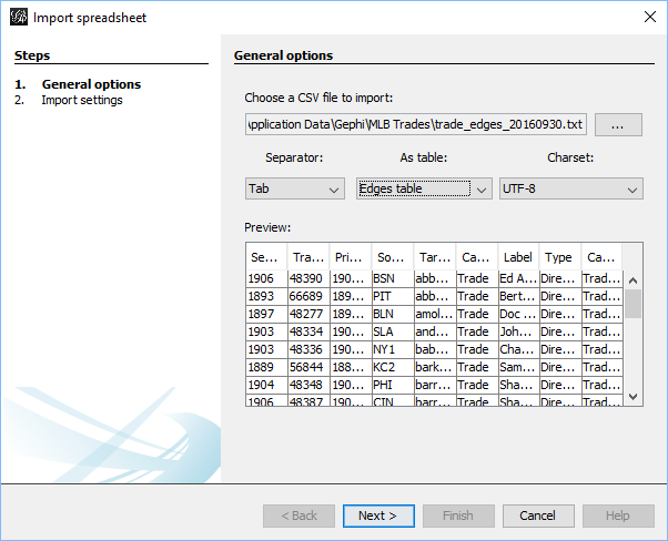
That’s it for our node creation process; the next post will share how we create the edges that will connect trades to teams and teams to players. Thanks for reading!

Major League Baseball Trade Networks, Part 2

Welcome to Part 2 in our miniseries on building baseball (MLB) trade networks with Gephi. In the first post, the focus was on procuring and preparing the data using MySQL. The goal was to create nodes and edges that could be easily imported to Gephi. Gephi does allow for some data manipulation post-import, but I’ve learned from experience to do the main parts of the job with either SQL code or within spreadsheet software like Excel or Calc.

With our data readied for import, we’ll now move on to the more fun parts of the process, where we get to visualize the data and see any underlying patterns. Gephi is an ideal tool for this, as it allows us to try out many different algorithms, especially in version 0.8.2. The newer 0.9 versions are faster, but have not fully caught up on the plugin side at this writing, so options are a bit more limited. One other caveat – I frequently run into Java issues when using Gephi, so save your work often and be prepared to shut down and restart Gephi periodically.

We’ll kick off this part of the process by importing the data, nodes first, followed by edges. The reason I prefer this order is that nodes will be automatically created if we start with the edge file import, and they won’t contain any extra fields you may have added using your database or spreadsheet processes.

Here’s the node import window, showing the appropriate file input:

Gephi node import window

Once the node import process is complete, we turn to the edges file, and follow a similar sequence of steps. Here’s our starting point:

Gephi edge import window

After the data has been imported, it’s time to move to the Overview tab, where we’ll see a dense mess of nodes and edges, especially if we have a fair sized dataset. Something like this:

Impossibly dense hairball network

Gephi offers a variety of interesting algorithms, each more or less appropriate based on the underlying dataset. In our case, the dataset is of a moderate size, with more than 8,000 nodes and nearly 62,000 edges. This immediately rules out the use of simple layouts such as the circular algorithms, as it would prove immensely challenging to display, even when we take it to an interactive output. At the other end of the sophistication level lie the force-directed layouts, which apply a significant dose of science and math within their respective algorithms. In Gephi, the Force Atlas 2 is quite popular, but it tends to run very slowly unless coupled with enormous levels of RAM. So where to go with our choice for this data?

I elected to take a two step approach, using the extremely fast (if less precise) OpenOrd algorithm for the original data. This provides a nice view of the network within a few minutes, making it a good starting point for our next steps.

Trade network with OpenOrd layout

The goal of this exercise was to create team level graphs, which will each have a small subset of the entire dataset. One easy way to achieve this is to use the Ego Network filter to select a single team and its connections. Setting the ego network to a depth of 1 limits the display to only first degree connections; in this case players traded to or from our selected team.

Ego network with depth = 1

Once this step has been taken, we can then refine the display by applying another algorithm; in this case I have chosen the Yifan Hu option, and adjusted the settings until they created an aesthetically pleasing graph. The Yifan Hu adds further precision within each of the team graphs, and provides them with a common look & feel inasmuch as their respective data allows.

We have now completed our basic graph creation in Gephi, and can output our results to a variety of output formats. Our choice here is to create a GEXF file, which we can then plug in to an existing template. We do have another step with respect to the GEXF data. In order to relate the graphs back to their respective teams, I chose to apply official team colors to elements in the graph. Specifically, each node should reflect the individual team; we want the edges to remain the same across all graphs so that users have a common understanding for the types of connections between players and teams. So to update the node colors, simply use a code editor that can perform batch updates. I typically work with Brackets for this task, but choose your tool of choice. Here’s a view of the GEXF output prior to applying color changes:

GEXF nodes with original colors

Now here’s the updated version that reflects the Tigers navy blue coloring:

GEXF nodes updated with team colors

Once this step has been completed, I can upload the files to the web server, where other minor changes can be made. These include any updates to the CSS styling, adjustments to the config.js file, and minor changes to the index.html file so the proper team information is displayed. The easiest way to do this is to create a common set of directories for the basic javascript and CSS files, leaving only the individual config, html, and gexf files in each team’s directory.

After a bit of massaging the config and CSS settings, the result is visually appealing as well as highly functional. Here’s a zoomed in look at the Toronto Blue Jays network on the web:

Blue Jays trade network close-up

All of the networks can be found by clicking the link below, with new ones being added until all teams have been represented:

Trade Networks

If you want to see each network in its own window or tab, use the right-click options in Firefox or Chrome.

I hope this has been helpful, and please feel free to reach out via the LinkedIn or Facebook Gephi groups, or leave a comment on this site.

Thanks for reading!