Category: Trade Networks

Major League Baseball Trade Networks, Part 2

Welcome to Part 2 in our miniseries on building baseball (MLB) trade networks with Gephi. In the first post, the focus was on procuring and preparing the data using MySQL. The goal was to create nodes and edges that could be easily imported to Gephi. Gephi does allow for some data manipulation post-import, but I’ve learned from experience to do the main parts of the job with either SQL code or within spreadsheet software like Excel or Calc.

With our data readied for import, we’ll now move on to the more fun parts of the process, where we get to visualize the data and see any underlying patterns. Gephi is an ideal tool for this, as it allows us to try out many different algorithms, especially in version 0.8.2. The newer 0.9 versions are faster, but have not fully caught up on the plugin side at this writing, so options are a bit more limited. One other caveat – I frequently run into Java issues when using Gephi, so save your work often and be prepared to shut down and restart Gephi periodically.

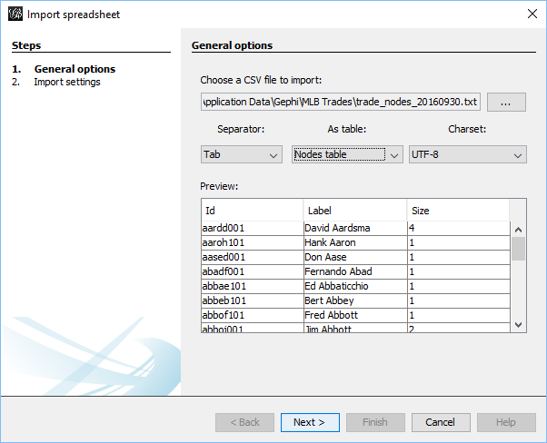
We’ll kick off this part of the process by importing the data, nodes first, followed by edges. The reason I prefer this order is that nodes will be automatically created if we start with the edge file import, and they won’t contain any extra fields you may have added using your database or spreadsheet processes.

Here’s the node import window, showing the appropriate file input:

Gephi node import window

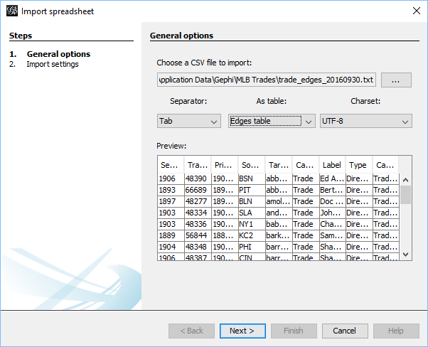
Once the node import process is complete, we turn to the edges file, and follow a similar sequence of steps. Here’s our starting point:

Gephi edge import window

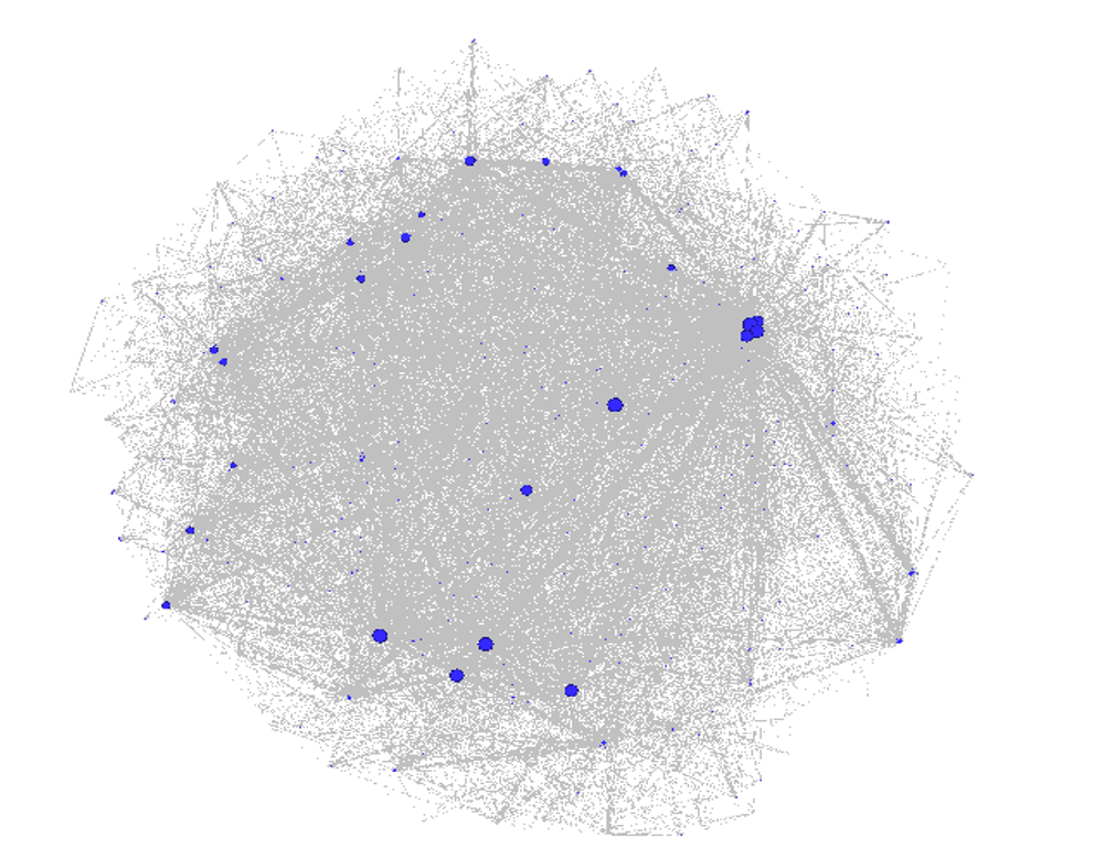
After the data has been imported, it’s time to move to the Overview tab, where we’ll see a dense mess of nodes and edges, especially if we have a fair sized dataset. Something like this:

Impossibly dense hairball network

Gephi offers a variety of interesting algorithms, each more or less appropriate based on the underlying dataset. In our case, the dataset is of a moderate size, with more than 8,000 nodes and nearly 62,000 edges. This immediately rules out the use of simple layouts such as the circular algorithms, as it would prove immensely challenging to display, even when we take it to an interactive output. At the other end of the sophistication level lie the force-directed layouts, which apply a significant dose of science and math within their respective algorithms. In Gephi, the Force Atlas 2 is quite popular, but it tends to run very slowly unless coupled with enormous levels of RAM. So where to go with our choice for this data?

I elected to take a two step approach, using the extremely fast (if less precise) OpenOrd algorithm for the original data. This provides a nice view of the network within a few minutes, making it a good starting point for our next steps.

Trade network with OpenOrd layout

The goal of this exercise was to create team level graphs, which will each have a small subset of the entire dataset. One easy way to achieve this is to use the Ego Network filter to select a single team and its connections. Setting the ego network to a depth of 1 limits the display to only first degree connections; in this case players traded to or from our selected team.

Ego network with depth = 1

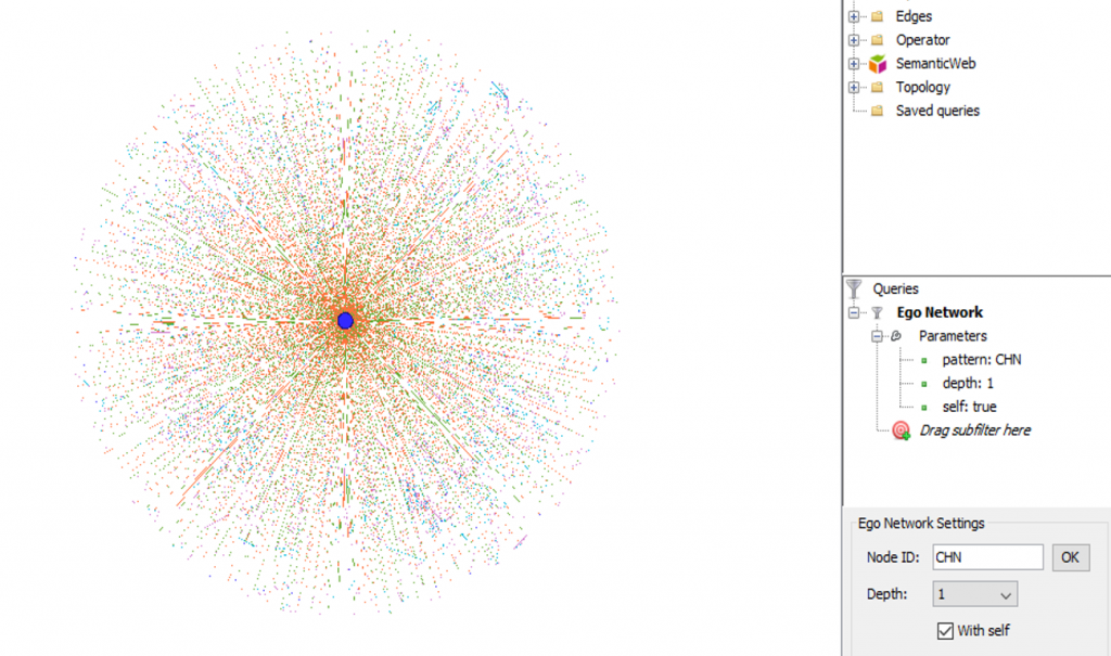
Once this step has been taken, we can then refine the display by applying another algorithm; in this case I have chosen the Yifan Hu option, and adjusted the settings until they created an aesthetically pleasing graph. The Yifan Hu adds further precision within each of the team graphs, and provides them with a common look & feel inasmuch as their respective data allows.

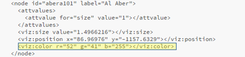
We have now completed our basic graph creation in Gephi, and can output our results to a variety of output formats. Our choice here is to create a GEXF file, which we can then plug in to an existing template. We do have another step with respect to the GEXF data. In order to relate the graphs back to their respective teams, I chose to apply official team colors to elements in the graph. Specifically, each node should reflect the individual team; we want the edges to remain the same across all graphs so that users have a common understanding for the types of connections between players and teams. So to update the node colors, simply use a code editor that can perform batch updates. I typically work with Brackets for this task, but choose your tool of choice. Here’s a view of the GEXF output prior to applying color changes:

GEXF nodes with original colors

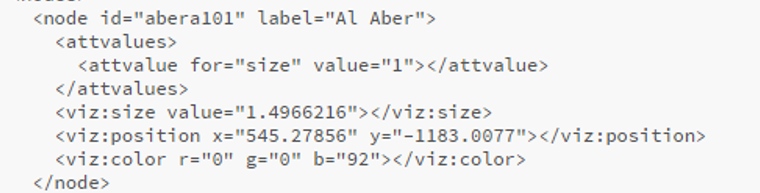
Now here’s the updated version that reflects the Tigers navy blue coloring:

GEXF nodes updated with team colors

Once this step has been completed, I can upload the files to the web server, where other minor changes can be made. These include any updates to the CSS styling, adjustments to the config.js file, and minor changes to the index.html file so the proper team information is displayed. The easiest way to do this is to create a common set of directories for the basic javascript and CSS files, leaving only the individual config, html, and gexf files in each team’s directory.

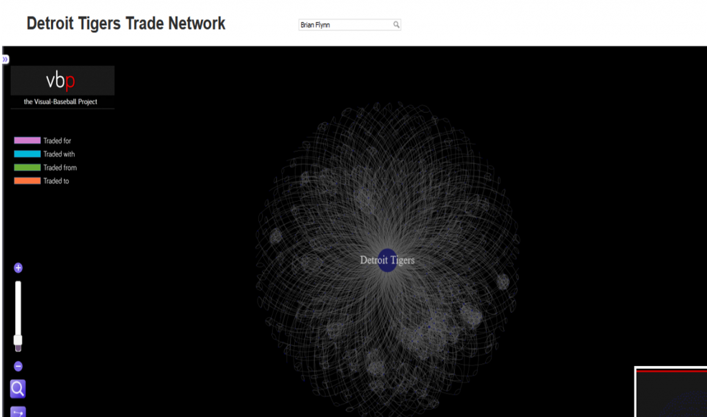
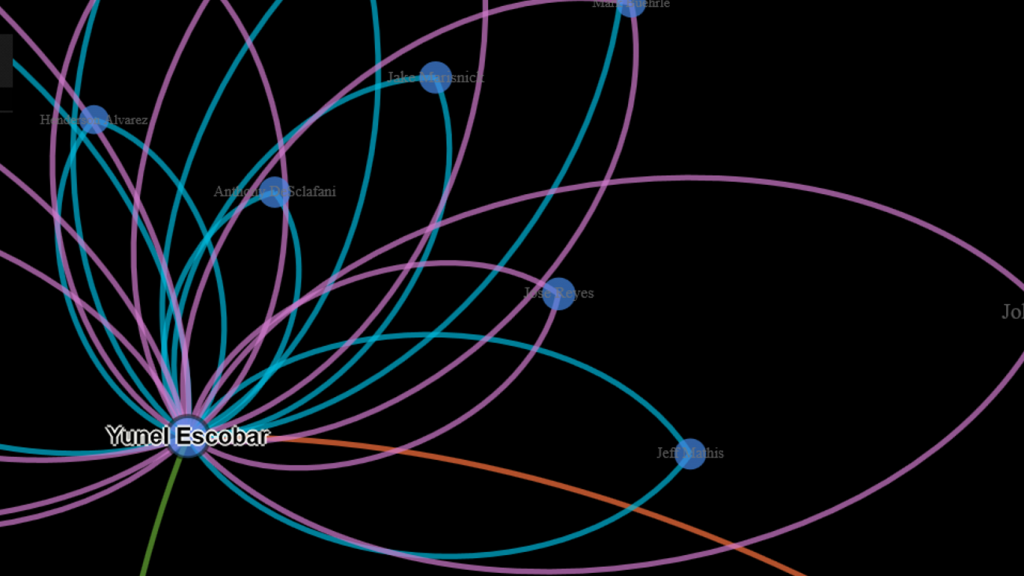
After a bit of massaging the config and CSS settings, the result is visually appealing as well as highly functional. Here’s a zoomed in look at the Toronto Blue Jays network on the web:

Blue Jays trade network close-up

All of the networks can be found by clicking the link below, with new ones being added until all teams have been represented:

Trade Networks

If you want to see each network in its own window or tab, use the right-click options in Firefox or Chrome.

I hope this has been helpful, and please feel free to reach out via the LinkedIn or Facebook Gephi groups, or leave a comment on this site.

Thanks for reading!

Major League Baseball Trade Networks, Part 1

One topic that has long fascinated me as network graph material is trade data between major league baseball (MLB) teams. I have previously created a static visualization showing activity at a macro level, i.e.- the number of trades between teams over a 100+ year period. Yet there was a desire to do something more, and to make it interactive so users would be able to sift through the data for their favorite teams to understand trade patterns through a visual representation. Today, after weeks spent tinkering with this topic, I finally have something to share, and will walk through how it is created and how to engage with it online. If you want to play with it before reading further, visit the Tigers trade network.

Here’s what we’ll wind up with:

Tigers trade network

My tools of choice in this endeavor are familiar ones to anyone working with baseball data, network graphs, or perhaps both, although I haven’t seen many instances of the latter. The trade data can be found at Retrosheet, as part of a seemingly boundless array of baseball data, both statistical and historical in nature. Gephi, the open source network analysis tool is again my choice for creating the network structure from the raw data, and Sigma.js is once more the tool for web implementation. Mix in a bit of Excel and PowerPoint for good measure, and we have all the tools necessary to create a pretty cool (IMHO) finished graph.

So let’s get started. Our first step is to go to the Retrosheeet site and download trade data, found at Retrosheet transactions. Be aware that there is much more than trade data in this dataset; free agent transactions, releases, and many other transaction types are available. My approach is to grab the entire dataset, which I can then load into a MySQL database for filtering and matching to other baseball data from both Retrosheet and the Lahman archives. For our example, only trades will be used; this leaves open the future possibility to examine free agent signings or other transaction types.

Once I have the data in MySQL (I’m purposely skipping over this process), the coding steps begin. This was a very iterative process as I gradually figured out how Gephi would play with the output data, but I won’t bore you with my multiple missteps. Instead, let’s have a look at the code snippets, and I’ll explain their usage and the thought process behind them. We’ll start with a view of the code, created within the (free) Toad for MySQL tool. In creating this code, we need to understand how Gephi (or other network analysis tools) work. At the risk of over-simplifying, Gephi only needs nodes and edges. Nodes will represent the players or teams in our visual, while edges will show the linkages within a single trade – who was traded for whom, and which players moved together from one organization to another.

Node creation is simple – we just grab all players involved in a trade, and do likewise for all teams. Here’s the code for players:

SELECT t.Player as Player, CONCAT(m.nameFirst, ” “, m.nameLast) as Name, count(*) as transactions

FROM trades2015 t
INNER JOIN Master m
ON t.Player = m.retroID

WHERE t.Type = ‘T’ and (t.TeamFrom > ‘A’ OR t.TeamTo > ‘A’)
GROUP BY t.Player, CONCAT(m.nameFirst, ” “, m.nameLast)

All we’re doing here is creating a node size for each player, based on the number of trades they are involved in.

For Teams, the logic is a bit more complex; since team names have changed from season to season, we need to join on both team and season to get the correct name assignments. We also want to account for the direction of each transaction, which we do using a UNION query.

SELECT b.Team AS Id, b.Name As Label, SUM(b.transactions) as Size
FROM
(SELECT t.TeamFrom as Team, te.name as Name, count(*) as transactions

FROM trades2015 t
INNER JOIN Teams te
ON te.teamID = t.TeamFrom and t.Season = te.yearID

WHERE t.Type = ‘T’ and t.TeamFrom > ‘A’
GROUP BY t.TeamFrom, te.name

UNION ALL

SELECT t.TeamTo as Team, te.name as Name, count(*) as transactions

FROM trades2015 t
INNER JOIN Teams te
ON te.teamID = t.TeamTo and t.Season = te.yearID

WHERE t.Type = ‘T’ and t.TeamFrom > ‘A’
GROUP BY t.TeamTo, te.name) b
GROUP BY b.Team, b.Name

After running the queries, we have results that can be posted into Excel or other spreadsheet software, where a tab-delimited file can be saved for use in Gephi. Our file data looks like this:

Id Label Size
aardd001 David Aardsma 4
aaroh101 Hank Aaron 1
aased001 Don Aase 1
abadf001 Fernando Abad 1
abbae101 Ed Abbaticchio 1
abbeb101 Bert Abbey 1
abbof101 Fred Abbott 1
abboj001 Jim Abbott 2

and for the team entries:


OAK Oakland Athletics 936
PH4 Philadelphia Athletics 6
PHA Philadelphia Athletics 355
PHI Philadelphia Blue Jays 28
PHI Philadelphia Phillies 1445
PHI Philadelphia Quakers 3
PIT Pittsburg Alleghenys 9
PIT Pittsburgh Pirates 1416

This is all Gephi requires for displaying nodes – an ID, a Label, and size. Even the label and size are not required fields, but they do make things easier if done in advance. So far, so good. Next we’ll move on to the somewhat more involved process of creating edge files.

As I progressed deeper into this project, it became evident to me that there were four different types of edges to display. The first two were obvious and easy – players being traded to a team, or from a team. Yet I also wanted to see the other players involved in each transaction, which necessitated the addition of two more edge type – traded with other players, and traded for other players. Note that in many cases just two or three of these might come into play, and for many prominent players, we’ll have none at all. Thus, the likes of an Al Kaline or Ted Williams will not be found in any of these graphs, as they remained with a single team for their entire careers.

Here’s the final edge code I wound up with to create the four categories of trades to be displayed in a graph. Gephi requires three edge attributes – a source value, a target value, and an edge type. The edge type must be either undirected or directed; for our graph, all edges will be directed, since we intend to show the bi-directional movements within each transaction. The first bit of code is for instances where a player was traded from a team:

SELECT tr.Season, tr.TransactionID, tr.PrimaryDate, tr.TeamFrom AS Source, tr.Player as Target,
CASE WHEN tr.Type = ‘T’ THEN ‘Trade’ WHEN tr.Type = ‘F’ THEN ‘Free Agent Signing’ WHEN tr.Type = ‘Fg’
THEN ‘Free Agent Granted’ WHEN tr.Type = ‘R’ THEN ‘Release’ END as Category,
CONCAT(m.nameFirst, ” “, m.nameLast, ” “, CASE WHEN tr.Type = ‘T’ THEN ‘Traded’ WHEN tr.Type = ‘F’ THEN ‘Free Agent Signing’ WHEN tr.Type = ‘Fg’
THEN ‘Free Agent Granted’ WHEN tr.Type = ‘R’ THEN ‘Released’ END, ” on “, tr.PrimaryDate, ” from “, t.name) AS Label, ‘Directed’ as Type, ‘Traded From’ as CategoryDetail

FROM trades2015 tr
INNER JOIN Master m ON tr.player = m.retroID
INNER JOIN Teams t ON tr.TeamFrom = t.teamIDretro and t.yearID = tr.season

WHERE tr.type = ‘T’

Note the legacy code covering free agency and releases, rendered moot by the WHERE clause. These will have to wait for another set of graphs. In a similar fashion we have code for trades where a player comes to a team.

SELECT tr.Season, tr.TransactionID, tr.PrimaryDate, tr.Player AS Source, tr.TeamTo as Target,
CASE WHEN tr.Type = ‘T’ THEN ‘Trade’ WHEN tr.Type = ‘F’ THEN ‘Free Agent Signing’ WHEN tr.Type = ‘Fg’
THEN ‘Free Agent Granted’ WHEN tr.Type = ‘R’ THEN ‘Release’ END as Category,
CONCAT(m.nameFirst, ” “, m.nameLast, ” “, CASE WHEN tr.Type = ‘T’ THEN ‘Traded’ WHEN tr.Type = ‘F’ THEN ‘Free Agent Signing’ WHEN tr.Type = ‘Fg’
THEN ‘Free Agent Granted’ WHEN tr.Type = ‘R’ THEN ‘Released’ END, ” on “, tr.PrimaryDate, ” to “, t.name) AS Label, ‘Directed’ as Type, ‘Traded To’ as CategoryDetail

FROM trades2015 tr
INNER JOIN Master m ON tr.player = m.retroID
INNER JOIN Teams t ON tr.TeamTo = t.teamIDretro and t.yearID = tr.season

WHERE tr.type = ‘T’

Next, it’s time to create linkages with players from the same transaction, first those moving in the same direction (traded with) in the trade.

SELECT tr.Season, tr.TransactionID, tr.PrimaryDate, tr.Player AS Source, tr2.Player AS Target,
CASE WHEN tr.Type = ‘T’ THEN ‘Trade’ WHEN tr.Type = ‘F’ THEN ‘Free Agent Signing’ WHEN tr.Type = ‘Fg’
THEN ‘Free Agent Granted’ WHEN tr.Type = ‘R’ THEN ‘Release’ END as Category,
CONCAT(m.nameFirst, ” “, m.nameLast, ” “, CASE WHEN tr.Type = ‘T’ THEN ‘Traded’ WHEN tr.Type = ‘F’ THEN ‘Free Agent Signing’ WHEN tr.Type = ‘Fg’
THEN ‘Free Agent Granted’ WHEN tr.Type = ‘R’ THEN ‘Released’ END, ” on “, tr.PrimaryDate, ” with “, m2.nameFirst, ” “, m2.nameLast) AS Label, ‘Directed’ as Type,
‘Traded With’ as CategoryDetail

FROM trades2015 tr
INNER JOIN trades2015 tr2
ON tr.TransactionID = tr2.TransactionID
INNER JOIN Master m ON tr.player = m.retroID
INNER JOIN Master m2 ON tr2.player = m2.retroID

WHERE tr.type = ‘T’

Note the need to duplicate the Master table in the code, since we now require multiple player names to populate the Source and Target fields in Gephi. The same holds true for our last snippet, where players are traded for one another.

SELECT tr.Season, tr.TransactionID, tr.PrimaryDate, tr.Player AS Source, tr2.Player AS Target,
CASE WHEN tr.Type = ‘T’ THEN ‘Trade’ WHEN tr.Type = ‘F’ THEN ‘Free Agent Signing’ WHEN tr.Type = ‘Fg’
THEN ‘Free Agent Granted’ WHEN tr.Type = ‘R’ THEN ‘Release’ END as Category,
CONCAT(m.nameFirst, ” “, m.nameLast, ” “,CASE WHEN tr.Type = ‘T’ THEN ‘Traded’ WHEN tr.Type = ‘F’ THEN ‘Free Agent Signing’ WHEN tr.Type = ‘Fg’
THEN ‘Free Agent Granted’ WHEN tr.Type = ‘R’ THEN ‘Released’ END, ” on “, tr.PrimaryDate, ” for “, m2.nameFirst, ” “, m2.nameLast) AS Label, ‘Directed’ as Type,
‘Traded For’ as CategoryDetail

FROM trades2015 tr
INNER JOIN trades2015 tr2
ON tr.TransactionID = tr2.TransactionID
INNER JOIN Master m ON tr.player = m.retroID
INNER JOIN Master m2 ON tr2.player = m2.retroID

WHERE tr.type = ‘T’

Each of these bits of code outputs results, which are then copied and pasted into our edges spreadsheet. Here are five rows showing each of our four trade categories:

Season TransactionID PrimaryDate Source Target Category Label Type CategoryDetail
2010 62908 20100731 KCA ankir001 Trade Rick Ankiel Traded on 20100731 from Kansas City Royals Directed Traded From
2010 60709 20100831 TEX ariaj001 Trade Joaquin Arias Traded on 20100831 from Texas Rangers Directed Traded From
2010 62264 20101118 COL barmc001 Trade Clint Barmes Traded on 20101118 from Colorado Rockies Directed Traded From
2010 72627 20101217 TBA bartj001 Trade Jason Bartlett Traded on 20101217 from Tampa Bay Rays Directed Traded From
2010 72622 20100709 TEX beavb001 Trade Blake Beavan Traded on 20100709 from Texas Rangers Directed Traded From

2010 62908 20100731 ankir001 ATL Trade Rick Ankiel Traded on 20100731 to Atlanta Braves Directed Traded To
2010 60709 20100831 ariaj001 NYN Trade Joaquin Arias Traded on 20100831 to New York Mets Directed Traded To
2010 62264 20101118 barmc001 HOU Trade Clint Barmes Traded on 20101118 to Houston Astros Directed Traded To
2010 72627 20101217 bartj001 SDN Trade Jason Bartlett Traded on 20101217 to San Diego Padres Directed Traded To
2010 72622 20100709 beavb001 SEA Trade Blake Beavan Traded on 20100709 to Seattle Mariners Directed Traded To

2010 62908 20100731 ankir001 blang001 Trade Rick Ankiel Traded on 20100731 for Gregor Blanco Directed Traded For
2010 62908 20100731 ankir001 chavj001 Trade Rick Ankiel Traded on 20100731 for Jesse Chavez Directed Traded For
2010 62908 20100731 ankir001 collt001 Trade Rick Ankiel Traded on 20100731 for Tim Collins Directed Traded For
2010 60709 20100831 ariaj001 franj004 Trade Joaquin Arias Traded on 20100831 for Jeff Francoeur Directed Traded For
2010 72627 20101217 bartj001 figuc001 Trade Jason Bartlett Traded on 20101217 for Cole Figueroa Directed Traded For

2010 62908 20100731 ankir001 farnk001 Trade Rick Ankiel Traded on 20100731 with Kyle Farnsworth Directed Traded With
2010 66840 20101219 betay001 greiz001 Trade Yuniesky Betancourt Traded on 20101219 with Zack Greinke Directed Traded With
2010 72622 20100709 beavb001 luekj001 Trade Blake Beavan Traded on 20100709 with Josh Lueke Directed Traded With
2010 72622 20100709 beavb001 smoaj001 Trade Blake Beavan Traded on 20100709 with Justin Smoak Directed Traded With
2010 62908 20100731 blang001 chavj001 Trade Gregor Blanco Traded on 20100731 with Jesse Chavez Directed Traded With

We have now successfully prepared the data for Gephi. In our next post, I’ll examine the process starting with the Gephi data import phase. Thanks for reading!

A New Book Resolution for 2016

As we enter a new year, I find myself eager to create a new book that explores the world of baseball data using a wide array of data visualization approaches. This idea has been in my head for several years at least, and has found partial fulfillment in my previously published pennant races book. However, I wish to tackle something broader that will touch a number of baseball categories as well as multiple data visualization approaches.

The working title for the book is ‘Baseball Grafika’, grafika being the Czech and Polish word for graphics, a word which still conveys the intent of the book regardless of language. If all goes well, the book will be available early in the 2016 baseball season, and will cover the following topics:

  • Franchise player networks
  • Trade pattern networks
  • Hall of Fame connection network
  • Franchise location maps
  • Player birthplace maps
  • Pennant race charts
  • Standings charts
  • Career trajectory graphs
  • Baseball dashboards

Fortunately, much work has been done over the last several years on at least a few of these topics, so we’re not starting from scratch, but this will still be a considerable, yet rewarding, challenge. Updates to come.