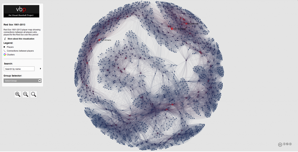
A few years back, I used Gephi and sigma.js to create a series of interactive baseball team networks, one for each current MLB franchise. These networks displayed all players through the 2013 season, going all the way back to 1901 for the original American and National League franchises. Now that we have data through the 2017 season, it’s time for an update, not only from a data perspective, but also stylistically. This post will walk through the process of creating one of these networks using Toad for MySQL, Gephi, and sigma.js to create web-based interactive network visualizations.
Here’s a typical network from the 2013 series; the full list of networks can be found here. We’ll use the existing networks as a baseline for the new networks, although a few modifications will be made.

Source Data & MySQL Queries
Let’s start our discussion with the source data. Season-level baseball data is available through the seanlahman.com website, in the form of .csv files or Microsoft Access database tables. I use the .csv format, as it can be easily added to existing MySQL databases on the visual-baseball.com server. MySQL also makes it simple to add derived fields through some simple coding. These fields can be utilized later for a variety of activities.
For the purpose of our network graphs, there are a handful of critical fields we want to use. These include the following:
- playerID, a unique identifier for every player who ever donned a major league uniform
- player name, which can be used to provide a meaningful reference based on the playerID field
- yearID, which refers to the season (or seasons) a player suited up for a specific franchise
- franchID, a unique identifier for each MLB franchise
We also need to do a little manipulation of the source data in our code to deliver our results in the proper form for use in Gephi. This means we need to create two input files – one for nodes, and a second for edges. The nodes will contain information about each player, the number of seasons played for the franchise and the first and last seasons, which may differ from the number of seasons, as players frequently leave a franchise only to return later in their career. Here’s our node code:
SELECT Id, Label, MAX(Size) as Size
FROM
(SELECT bp.playerID AS Id, CONCAT(bp.name, ” “, MIN(bp.yearID), “-“, MAX(bp.yearID)) AS Label, COUNT(bp.yearID) AS Size
FROM BattingPlus bp
WHERE bp.franchID = ‘BOS’ and bp.yearID >= 1901
GROUP BY bp.name
UNION ALL
SELECT pp.playerID AS Id, CONCAT(pp.name, ” “, MIN(pp.yearID), “-“, MAX(pp.yearID)) AS Label, COUNT(pp.yearID) AS Size
FROM BattingPlus pp
WHERE pp.franchID = ‘BOS’ and pp.yearID >= 1901
GROUP BY pp.name) a
GROUP BY Id
ORDER BY Id;
Here’s the simple interpretation – since we are attempting to display all players for a given franchise, we are executing a UNION ALL statement to combine batters and pitchers into a single result file. We have used the playerID field to create the required Id value for Gephi, while also creating a Label field by combining the player’s name with their first and last years playing for this franchise. Finally, we have created a Size field based on the number of seasons played for the franchise. We can then choose to use this in Gephi to size each node, if we so choose.
We also need to create the edge file for Gephi. In this case, we want to understand how many seasons two players were on the same team. This code is a bit trickier, since we want to show only one connection between two players, since this will be an undirected graph. More on that distinction later. Here’s our edge code:
SELECT b.playerID AS Source, m.playerID AS Target, ‘Undirected’ as Type, ‘ ‘ as Id, ‘ ‘ as Label, count(*) as weight
FROM
(SELECT a.playerID, CONCAT(m.nameFirst, ” “, m.nameLast) name, a.yearID, a.franchID
FROM Appearances a
INNER JOIN Master m
ON a.playerID = m.playerID
WHERE a.franchID = ‘BOS’ and a.yearID >= 1901) b
INNER JOIN Appearances a
ON b.yearID = a.yearID and b.franchID = a.franchID and b.playerID <> a.playerID and a.playerID > b.playerID
INNER JOIN Master m
ON a.playerID = m.playerID
GROUP BY b.playerID, a.playerID
ORDER BY b.playerID
Here we use the Master table to provide player name information, and we also gather the ID information to match the node values. The critical piece in this code is in our join criteria:
INNER JOIN Appearances a
ON b.yearID = a.yearID and b.franchID = a.franchID and b.playerID <> a.playerID and a.playerID > b.playerID
Here we are matching players based on the same season and the same franchise. We then specify that we do not want to connect any player to himself, and that we want only values where the playerID value from our main query is greater than the playerID value from the sub-query. This gives us a single connection between two players, which is what we need for an undirected graph. We then define a Source node (required by Gephi) and a Target node (also required), as well as specifying ‘Undirected’ as the graph type. We leave the ID and Label values empty, and then summarize the number of seasons played together as an edge weight. This value can be used in Gephi to show the strength of a connection between two nodes (e.g.- did they spend one season together, or 10 seasons together?).
After exporting each of these files to a .csv format, we have our source data for Gephi. In Part 2 our focus will shift to creating the network in Gephi.